Multimodal RAG for processing videos using OpenAI GPT4V and LanceDB vectorstore#

In this notebook, we showcase a Multimodal RAG architecture designed for video processing. We utilize OpenAI GPT4V MultiModal LLM class that employs CLIP to generate multimodal embeddings. Furthermore, we use LanceDBVectorStore for efficient vector storage.

Steps:

Download video from YouTube, process and store it.
Build Multi-Modal index and vector store for both texts and images.
Retrieve relevant images and context, use both to augment the prompt.
Using GPT4V for reasoning the correlations between the input query and augmented data and generating final response.

%pip install llama_index ftfy regex tqdm
%pip install git+https://github.com/openai/CLIP.git
%pip install torch torchvision
%pip install matplotlib scikit-image
%pip install lancedb
%pip install moviepy
%pip install pytube
%pip install pydub
%pip install SpeechRecognition
%pip install ffmpeg-python

from moviepy.editor import VideoFileClip
from pydub import AudioSegment
from pathlib import Path
import speech_recognition as sr
from pytube import YouTube
from pprint import pprint

import os

OPENAI_API_TOKEN = ""
os.environ["OPENAI_API_KEY"] = OPENAI_API_TOKEN

Set configuration for input below#

video_url = "https://www.youtube.com/watch?v=d_qvLDhkg00"
output_video_path = "./video_data/"
output_folder = "./mixed_data/"
output_audio_path = "./mixed_data/output_audio.wav"

filepath = output_video_path + "input_vid.mp4"
Path(output_folder).mkdir(parents=True, exist_ok=True)

Download and process videos into appropriate format for generating/storing embeddings#

from PIL import Image
import matplotlib.pyplot as plt
import os


def plot_images(image_paths):
    images_shown = 0
    plt.figure(figsize=(16, 9))
    for img_path in image_paths:
        if os.path.isfile(img_path):
            image = Image.open(img_path)

            plt.subplot(2, 3, images_shown + 1)
            plt.imshow(image)
            plt.xticks([])
            plt.yticks([])

            images_shown += 1
            if images_shown >= 7:
                break

def download_video(url, output_path):
    """
    Download a video from a given url and save it to the output path.

    Parameters:
    url (str): The url of the video to download.
    output_path (str): The path to save the video to.

    Returns:
    dict: A dictionary containing the metadata of the video.
    """
    yt = YouTube(url)
    metadata = {"Author": yt.author, "Title": yt.title, "Views": yt.views}
    yt.streams.get_highest_resolution().download(
        output_path=output_path, filename="input_vid.mp4"
    )
    return metadata


def video_to_images(video_path, output_folder):
    """
    Convert a video to a sequence of images and save them to the output folder.

    Parameters:
    video_path (str): The path to the video file.
    output_folder (str): The path to the folder to save the images to.

    """
    clip = VideoFileClip(video_path)
    clip.write_images_sequence(
        os.path.join(output_folder, "frame%04d.png"), fps=0.2
    )


def video_to_audio(video_path, output_audio_path):
    """
    Convert a video to audio and save it to the output path.

    Parameters:
    video_path (str): The path to the video file.
    output_audio_path (str): The path to save the audio to.

    """
    clip = VideoFileClip(video_path)
    audio = clip.audio
    audio.write_audiofile(output_audio_path)


def audio_to_text(audio_path):
    """
    Convert audio to text using the SpeechRecognition library.

    Parameters:
    audio_path (str): The path to the audio file.

    Returns:
    test (str): The text recognized from the audio.

    """
    recognizer = sr.Recognizer()
    audio = sr.AudioFile(audio_path)

    with audio as source:
        # Record the audio data
        audio_data = recognizer.record(source)

        try:
            # Recognize the speech
            text = recognizer.recognize_whisper(audio_data)
        except sr.UnknownValueError:
            print("Speech recognition could not understand the audio.")
        except sr.RequestError as e:
            print(f"Could not request results from service; {e}")

    return text

try:
    metadata_vid = download_video(video_url, output_video_path)
    video_to_images(filepath, output_folder)
    video_to_audio(filepath, output_audio_path)
    text_data = audio_to_text(output_audio_path)

    with open(output_folder + "output_text.txt", "w") as file:
        file.write(text_data)
    print("Text data saved to file")
    file.close()
    os.remove(output_audio_path)
    print("Audio file removed")

except Exception as e:
    raise e

Moviepy - Writing frames ./mixed_data/frame%04d.png.

Moviepy - Done writing frames ./mixed_data/frame%04d.png.
MoviePy - Writing audio in ./mixed_data/output_audio.wav

MoviePy - Done.
Text data saved to file
Audio file removed

Use index as retriever to fetch top k (5 in this example) results from the multimodal vector index#

retriever_engine = index.as_retriever(
    similarity_top_k=5, image_similarity_top_k=5
)

Set the RAG prompt template#

import json

metadata_str = json.dumps(metadata_vid)

qa_tmpl_str = (
    "Given the provided information, including relevant images and retrieved context from the video, \
 accurately and precisely answer the query without any additional prior knowledge.\n"
    "Please ensure honesty and responsibility, refraining from any racist or sexist remarks.\n"
    "---------------------\n"
    "Context: {context_str}\n"
    "Metadata for video: {metadata_str} \n"
    "---------------------\n"
    "Query: {query_str}\n"
    "Answer: "
)

Retrieve most similar text/image embeddings baseed on user query from the DB#

from llama_index.response.notebook_utils import display_source_node
from llama_index.schema import ImageNode


def retrieve(retriever_engine, query_str):
    retrieval_results = retriever_engine.retrieve(query_str)

    retrieved_image = []
    retrieved_text = []
    for res_node in retrieval_results:
        if isinstance(res_node.node, ImageNode):
            retrieved_image.append(res_node.node.metadata["file_path"])
        else:
            display_source_node(res_node, source_length=200)
            retrieved_text.append(res_node.text)

    return retrieved_image, retrieved_text

Add query now, fetch relevant details including images and augment the prompt template#

query_str = "Using examples from video, explain all things covered in the video regarding the gaussian function"

img, txt = retrieve(retriever_engine=retriever_engine, query_str=query_str)
image_documents = SimpleDirectoryReader(
    input_dir=output_folder, input_files=img
).load_data()
context_str = "".join(txt)
plot_images(img)

Node ID: 2b0dab05-1469-48a2-9f36-2103458ba252
Similarity: 0.742850661277771
Text: The basic function underlying a normal distribution, aka a Gaussian, is e to the negative x squared. But you might wonder why this function? Of all the expressions we could dream up that give you s…

Node ID: 6856d43b-9978-4882-a1ff-09d11913157b
Similarity: 0.7337126731872559
Text: This step is actually pretty technical, it goes a little beyond what I want to talk about here. Often use these objects called moment generating functions, that gives you a very abstract argument t…

Node ID: 27e3d1f6-4b30-4087-a93d-5484edc814d3
Similarity: 0.7068501114845276
Text: This is the important point. All of the stuff that’s involving s is now entirely separate from the integrated variable. This remaining integral is a little bit tricky. I did a whole video on it. It…

Node ID: 320ed2fc-eeaa-48a3-a216-b90e0316b1a8
Similarity: 0.7065496444702148
Text: The essence of what we want to compute is what the convolution between two copies of this function looks like. If you remember, in the last video, we had two different ways to visualize convolution…

../../_images/795c4f58cb6319504a52b6a53c7e7864d26d583743072bfbf0c1dd1655fc7546.png

Generate final response using GPT4V#

from llama_index.multi_modal_llms.openai import OpenAIMultiModal

openai_mm_llm = OpenAIMultiModal(
    model="gpt-4-vision-preview", api_key=OPENAI_API_TOKEN, max_new_tokens=1500
)


response_1 = openai_mm_llm.complete(
    prompt=qa_tmpl_str.format(
        context_str=context_str, query_str=query_str, metadata_str=metadata_str
    ),
    image_documents=image_documents,
)

pprint(response_1.text)

('The video titled "A pretty reason why Gaussian + Gaussian = Gaussian" by '
 '3Blue1Brown covers several aspects of the Gaussian function, also known as '
 'the normal distribution. Here are the key points discussed in the video:\n'
 '\n'
 '1. **Central Limit Theorem**: The video begins by discussing the central '
 'limit theorem, which states that the sum of multiple copies of a random '
 'variable tends to look like a normal distribution. As the number of summed '
 'variables increases, the approximation to a normal distribution becomes '
 'better.\n'
 '\n'
 '2. **Convolution of Random Variables**: The process of adding two random '
 'variables is mathematically represented by a convolution of their respective '
 'distributions. The video explains how to visualize the convolution operation '
 'using two methods, with a focus on the second method involving diagonal '
 'slices.\n'
 '\n'
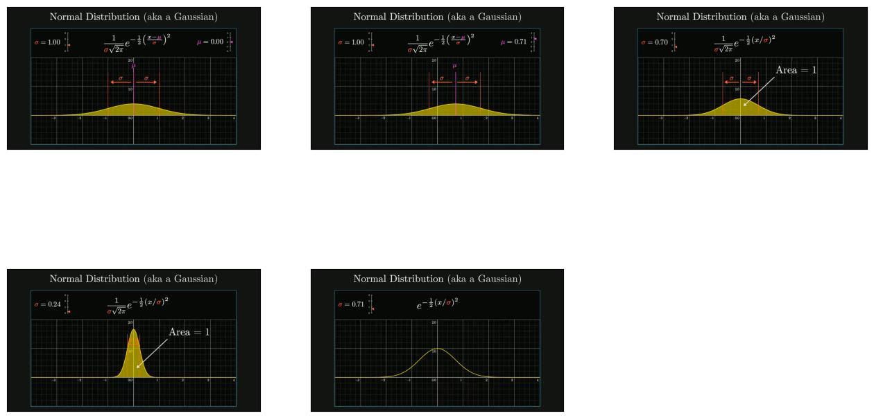
 '3. **Gaussian Function**: The Gaussian function is more complex than just '
 '\\(e^{-x^2}\\). The full formula includes a normalization factor to ensure '
 'the area under the curve is one, making it a valid probability distribution. '
 'The standard deviation (\\(\\sigma\\)) is used to describe the spread of the '
 'distribution, and the mean (\\(\\mu\\)) can be included to shift the center '
 'of the distribution.\n'
 '\n'
 '4. **Convolution of Two Gaussians**: The video explores what happens when '
 'you add two normally distributed random variables, which is equivalent to '
 'computing the convolution of two Gaussian functions. The author presents a '
 'visual approach to understand this calculation by exploiting the rotational '
 'symmetry of the graph of \\(e^{-x^2}\\).\n'
 '\n'
 '5. **Rotational Symmetry and Slices**: The video demonstrates that the graph '
 'of \\(e^{-x^2} \\cdot e^{-y^2}\\) is rotationally symmetric around the '
 'origin, which is a unique property of Gaussian functions. By examining '
 'diagonal slices of this graph, the author shows how to compute the area '
 'under these slices, which corresponds to the convolution of the two '
 'functions.\n'
 '\n'
 '6. **Resulting Distribution**: The convolution of two Gaussian functions is '
 'shown to be another Gaussian function. This is a special property because '
 'convolutions typically result in a different kind of function. The video '
 'explains that this property is key to understanding why the Gaussian '
 'function is the universal shape approached by the central limit theorem.\n'
 '\n'
 '7. **Standard Deviation of the Result**: When reintroducing the constants '
 'for a normal distribution, the video concludes that the convolution of two '
 'normal distributions with mean 0 and standard deviation \\(\\sigma\\) '
 'results in another normal distribution with a standard deviation of '
 '\\(\\sqrt{2} \\cdot \\sigma\\).\n'
 '\n'
 '8. **Implications for the Central Limit Theorem**: The video emphasizes that '
 'the computation of the convolution of two Gaussians is fundamental to the '
 'central limit theorem. It shows that the Gaussian distribution is a fixed '
 'point in the space of distributions, which is why it is the shape that '
 'emerges from the central limit theorem.\n'
 '\n'
 'Throughout the video, the author provides visual examples and explanations '
 'to help viewers understand the mathematical concepts involved in the '
 'Gaussian function and its properties related to probability and statistics.')